HISTORY OF REMOTE SENSING, SATELLITE IMAGERY,
PART II
COPYRIGHT © 2009 Paul R. Baumann
INTRODUCTION:
The period from 1960 to 2010 has experienced some major changes in the field of remote sensing. The background for many of these changes occurred in the 1960s and 1970s. Some of these changes are outlined below.
First, the term “remote sensing” was initially introduced in 1960. Before 1960 the term used was generally aerial photography. However, new methods and technologies for sensing of the Earth’s surface were moving beyond the traditional black and white aerial photograph, requiring a new, more comprehensive term be established.
Second, the 1960s and 1970s saw the primary platform used to carry remotely sensed instruments shift from air planes to satellites. Satellites can cover much more land space than planes and can monitor areas on a regular basis.
Third, imagery became digital in format rather than analog. The digital format made it possible to display and analyze imagery using computers, a technology that was also undergoing rapid change during this period. Computer technology was moving from large mainframe machines to small microcomputers and providing information more in graphic form rather than numerical output.
Fourth, sensors were becoming available that recorded the Earth’s surface simultaneously in several different portions of the electro-magnetic spectrum. One could now view an area by looking at several different images, some in portions of the spectrum beyond what the human eye could view. This technology made it possible to see things occurring on the Earth’s surface that looking at a normal aerial photograph one could not detect.
Finally, the turbulent social movements of the 1960s and 1970s awakened a new and continuing concern about the changes in the Earth’s physical environment. Remotely sensed imagery from satellites - analyzed and enhanced with computers - made it possible to detect and monitor these changes. Thus, societal support was and continues to remain strong for this technology, even though very few people are familiar with the term, remote sensing.
Today, many satellites, with various remote sensing instruments, monitor the Earth’s surface. These satellites and their respective remote sensing programs can trace their origins back to the CORONA and Landsat programs. CORONA was a secretive military reconnaissance program that continues to the present time through the advanced Keyhole satellites and Landsat was an open Earth resources program that also continues through more advanced Landsats and other satellite resource monitoring programs. This unit centers on the development and growth of these two programs.
CORONA: AMERICA’S FIRST SATELLITE PROGRAM
The CORONA Program occurred between 1959 and 1972 but the American public did not know about the project until 1995 when President Bill Clinton ordered the declassification of the imagery. Vice President Al Gore urged the declassification of the imagery in order to assist scientists in conducting various environmental studies.
U-2 Aircraft Reconnaissance Program
To appreciate the importance of the CORONA Program some historical context is required. After World War II and through the 1950s, the Cold War with the Soviet Union created a need for the United States to know about the military strength of the Soviet Union, especially with respect to the number of long range bombers and intercontinental ballistic missiles (ICBMs) that it possessed. Reconnaissance planes were being sent across the borders into the Soviet Union and its allied nations. However, these planes could only penetrate the edges of the country and the information needed was in the middle of the Soviet Union’s large land mass. Many of these planes and their crews never returned. A new plane was required that could fly high enough that Soviet planes and surface-to-air missiles could not shoot it down. More importantly this plane needed to be able to take detailed aerial photographs over the middle of the Soviet Union.
In 1954, President Dwight Eisenhower had the CIA, working in conjunction with the U.S. Air Force, negotiate an arrangement with Lockheed to create such an airplane. This arrangement led to the development of the secret Lockheed Skunk Works where Kelly Johnson and his engineers created within a few months the U-2. Eisenhower realized that the use of such a plane over the territory of another nation was in violation of the other nation’s sovereignty and could result in military reprisal. However, he was under pressure from the military-industrial complex in the United States to address the supposed large bombe and ICBM advantage that the Soviet Union had over the U.S. and the verbal threats being made by the Soviet leadership. Before using such a plane he proposed to the Soviet Union that both countries be allowed to send reconnaissance planes across each other’s territory in order to permit each country to have accurate information about the other country’s military strength. This proposal was rejected by the Soviet Union.
The first overflight of the Soviet Union by a U-2 occurred on July 4, 1956. It took off from West Germany and flew over Poland, Belorussia, Moscow, Leningrad, and the Soviet Baltic states. It flew at 70,000 feet, about 25,000 feet higher than any other plane could fly at the time, and exposed 3,600 feet of film per mission using two high-resolution cameras. One camera had a long focal length allowing it to spot items that were two to three feet across. These flights occurred several times over the next few years followed each time by formal protests by the Soviet Union. U-2 flights were also made over other nations. Finally, on May 1, 1960, using a cluster of 14 SA-2 missiles, the Soviet Union was able to shoot down a U-2 over its territory. The plane’s pilot, Francis Gary Powers, survived, and in August 1960 the Soviets staged a highly publicized trial to embarrass the United States. The United States agreed never to fly a reconnaissance plane across the Soviet Union again. This agreement included Communist China and Eastern Europe. These countries became known as the “denied areas.” The U-2 flights over the Soviet Union showed that no bomber or missile gap existed. Based on this information Eisenhower, an ex-military man, warned the nation immediately before leaving the presidency about the influence of the military-industrial complex and its role in shaping U.S. policy. It was the pressure from this complex that lead to the development of the U-2 and the possible conflict with the Soviet Union. The U-2 was later used in other sections of the world, most noticeably Cuba and Vietnam.
Figure 1 is an aerial photograph taken from a U-2 of a long range bomber airfield in the Soviet Union. The number of bombers can be counted as they are arranged along the length of the field. Several open spaces exist along the alignment suggesting parking areas for planes that might be in flight. Two bombers are located in the upper left side of the photo and can easily taxi to the runway for a quick takeoff. A bomber also appears to be located in the midfield. At both ends of the airfield are smaller planes, probably fighters to protect the airfield from attack. The bombers are most likely the Tupolev Tu-95, a large, four-engine turboprop powered plane that was both a long range bomber and missile platform. Its distinctively swept back wings are at 35 degrees, a very sharp angle by the standards of propeller-driven aircraft.
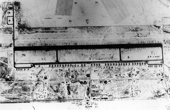
FIGURE 1: U-2 aerial photograph of an airfield in the Soviet Union.
CORONA Program
From the beginning of the U-2 program it was recognized that within a short time the Soviet Union would find a way to bring down a U-2; thus, the United States embarked in 1956, about the time of the first flight of a U-2 over the Soviet Union, to develop a reconnaissance system based on orbiting satellites. This system would be later called CORONA. On August 19, 1960, when Powers was on trial, the first successful air catch was made of a capsule of exposed film ejected from a photographic reconnaissance satellite. The satellite had made seven passes over the denied territory and 17 orbits of the Earth. From this imagery 64 Soviet airfields and 26 new surface-to-air (SAM) sites were identified. Satellites were not included in the agreement creating the denied territory. When the Soviets launched Sputnik I in 1957, they effectively established a worldwide “open skies” policy for items placed in orbit. The effort to launch a camera carrying satellite and recover imagery from it represented four years of intensive and frequently frustrating work. However, when the first successful CORONA satellite system occurred in 1960 it started the age of space reconnaissance and revolutionized remote sensing. One CORONA mission recorded more photographic coverage than all of the U-2 missions
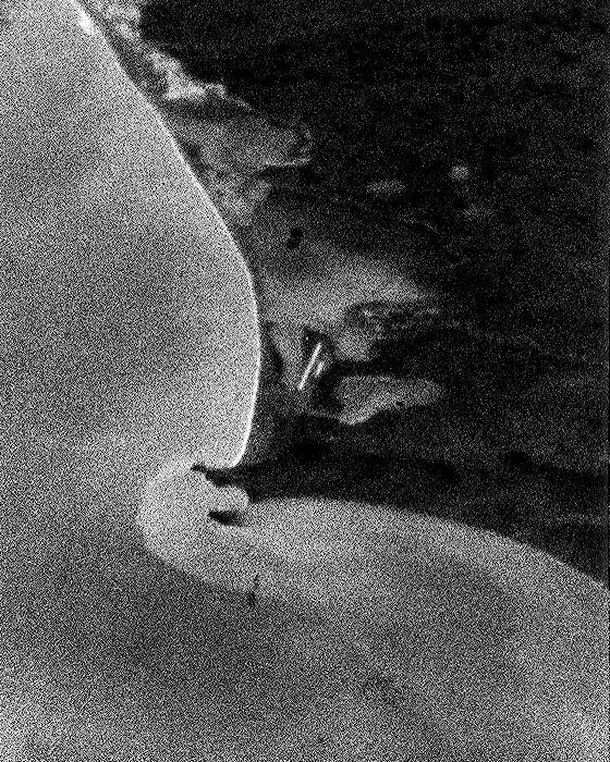
FIGURE 2: First CORONA photograph.
Figure 2 is the first CORONA reconnaissance photograph. Taken on August 8, 1960, it shows the Mys Shmidta Air Field, U.S.S.R. Both the runway and parking apron can be identified. In comparison to the U-2 photograph, the image lacks detail. This is due to the ground resolution being 40ft by 40ft. However, the situation was rectified within a few years with the KH-4 having a 5ft by 5ft resolution. See the detail on Figure 3 (KH-4 image), showing the Soviet Airfield, Minerallye Vod. The quality of this photograph is as good as the U-2 photograph, which is rather remarkable since it was taken about 10 times higher in altitude than the U-2 photograph.
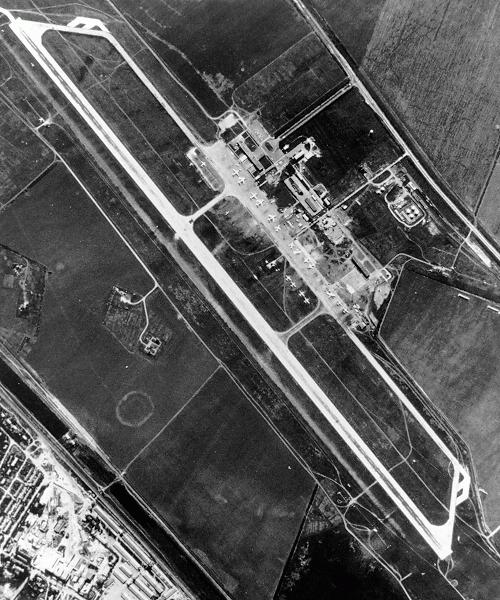
FIGURE 3: CORONA 4 photograph of Soviet airfield.
Table 1: Summary of CORONA Program – 1959 to 1972
| Camera | Launches | Recoveries | Time Period | |
| KH-1 | 10 | 1 | 1959-1960 | |
| KH-2 | C'(C Prine) | 10 | 4 | 1960-1961 |
| KH-3 | C''' (C Triple Prime) | 6 | 5 | 1961-1962 |
| KH-4 | M (Mural) | 26 | 20 | 1962-1963 |
| KH-4A | J (J-1) | 52 | 94 | 1964-1969 |
| KH-4B | J-3 | 17 | 32 | 1967-1972 |
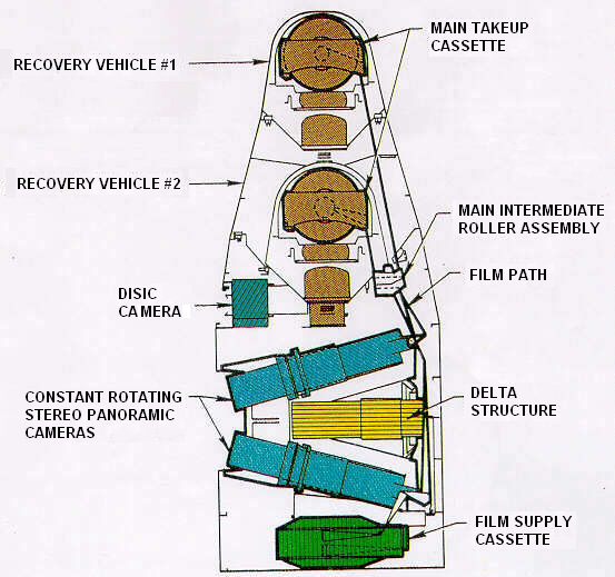
FIGURE 4: Stereo panoramic camera system used on KH-4A missions.
The first four versions of CORONA were designated KH-1 through KH-4 (Table 1). KH denoted Keyhole. The KH naming system was first used in 1962 with KH-4, with earlier numbers being retroactively applied. The public cover name for CORONA was DISCOVERER, a program that was supposed to be conducting scientific experiments. The KH-1 carried a single panoramic camera that had a ground resolution (the smallest visible ground area detected from the satellite) of 40 ft by 40 ft. The KH-2 and KH-3 missions also had single panoramic cameras but with a resolution of 10 ft by 10 ft. The KH-4, KH-4A, and KH-4B missions carried two panoramic cameras with a 30 degrees separation angle (Figure 4). This allowed for the creation of stereoscopic images, which permitted analysts to look at ground features from a three-dimensional perspective. By 1967 the KH-4s had cameras recording imagery at a 5 ft by 5 ft resolution.

FIGURE 5: Satellite capsule being captured.
The satellites were designed to release film canisters in capsules, called "buckets", which were recovered in mid-air by a specially equipped aircraft during their parachute descent (Figure 5). They were designed to float in water for a short period of time, and then sink, if the mid-air recovery failed. Early missions operated with a single bucket, but starting with KH-4A two buckets were available. The CORONA satellites used 31,500 ft (9,600 m) of special 70 mm film with a 24 inch (0.6 m) focal length lens. The CORONA Program continued until 1972 with the last image taken on May 31. Over 800,000 images were acquired. There were 121 launches and 156 recoveries.
Two other systems, closely related to CORONA, operated during this time period. The KH-5 (ARGON) was prepared for the Army mapping services during the early 1960s and the KH-6 (LANYARD) was designed to test a very high resolution camera systems. The KH-6 system was based on the success of KH-5, which produced disappointing results. Consequently both systems were terminated in 1963.
In 1967, President Lyndon Johnson, in a talk to a group of educators, responded to criticism that too much was being spent on space endeavors and not enough on the War on Poverty by saying:
“I wouldn’t want to be quoted on this, but we’ve spent thirty-five or forty billion dollars on the space program. And if nothing else had come out of it except the knowledge we’ve gained from space photography, it would be worth ten times what the whole program has cost. Without satellites, I’d be operating by guess. But tonight we know how many missiles the enemy has, and it turned out our guesses were way off. We were doing things we didn’t need to do. We were building things we didn’t need to build. We were harboring fears we didn’t need to harbor.” (Jensen)
This talk was based on imagery obtained from CORONA KH-4 satellites.
Even though the KH-1 through KH-4 satellites provided valuable information, they possessed some problems. The operation of retrieving the film capsules that were parachuted back to the Earth and snagged in mid-air by a plane was not always successful. This was especially the case with the KH-1 and KH-2 recoveries. Also, it might take days or weeks after the film was exposed before a capsule was released. Some events such as the 1967 Middle East Six-Day War and the 1968 Soviet invasion of Czechoslovakia were time sensitive and ended before imagery was available.
Although the CORONA Program was completed in 1972, the Keyhole reconnaissance satellites continue with the present KH-13s. The new Keyhole satellites have real time coverage, are able to record images at night, and transfer digital images electronically; thus, they can provide immediate imagery at any time. Little is known about the KH-13 satellites other than there appears to be several orbiting the Earth at the present time and two of them might be stealth in design. Figure 6 is an artist’s view of what a KH-12 might have looked liked.
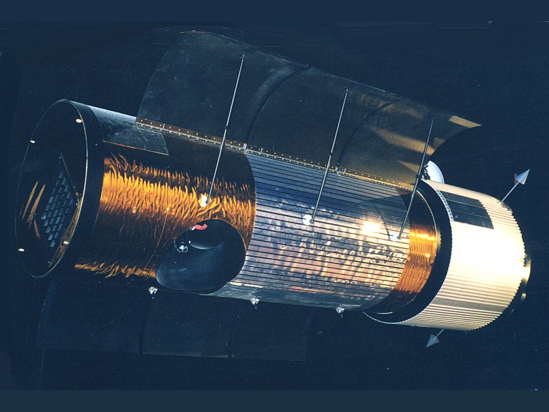
FIGURE 6: Artist rendition of a KH-12 satellite.
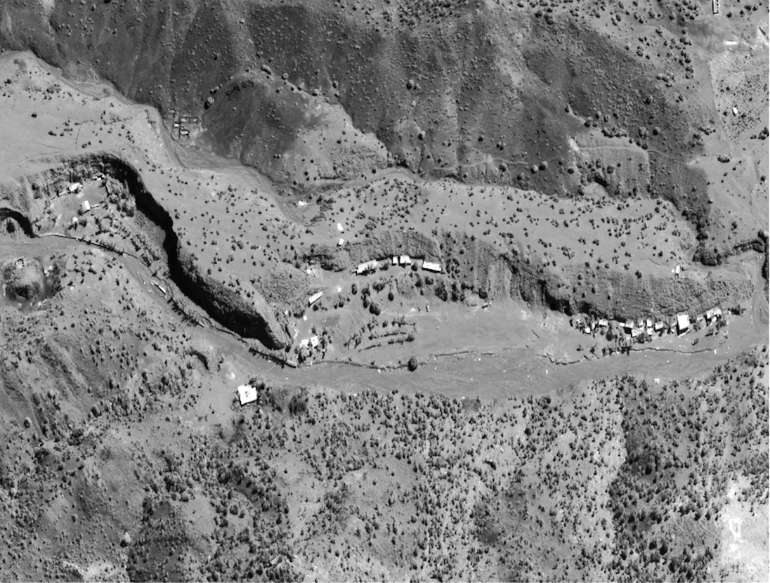
FIGURE 7: Zhawar Kili support complex in Afghanistan
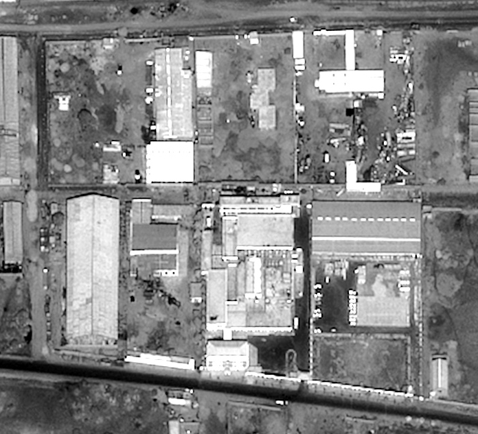
FIGURE 8: Shifa pharmaceutical plant, Sudan.
Figure 7 is a photograph taken of the Taliban Zhawar Kili Support Complex in Afghanistan supposedly recorded from a KH-12. More than likely the actual photograph provides much more detail than provided in this figure. Figure 7 and 8 were used by Secretary of Defense William S. Cohen and Gen. Henry H. Shelton, U.S. Army, chairman, Joint Chiefs of Staff, to brief reporters in the Pentagon on the U.S. military strike on a chemical weapons plant in Sudan and terrorist training camps in Afghanistan on Aug. 20, 1998.
Figure 9 is an image of the Fernsehturm Tower (German for "television tower") in Berlin taken on June 2008 by the commercial satellite, QuickBird. One can easily detect items as small as cars. KH-13 satellites must have considerably greater resolution than what can be obtained from a commercial satellite. Reports have been made that the resolution is great enough to read the license plates on cars.
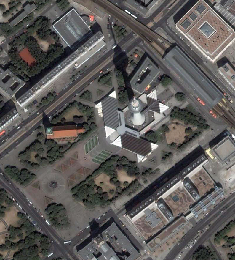
FIGURE 9: Image of Berlin’s Fernsehturm Tower taken June 2008 by the QuickBird satellite.
While the United States has been recording events over the Soviet Union from space, the Soviets were doing the same thing over the United States. The Soviet Union launched its reconnaissance satellite system in 1961 with the Zenit-2 program. Designed differently from the CORONA Program, it also obtained good imagery. Thus, Eisenhower’s proposal of allowing each nation to have reconnaissance flights over each other's air space became effective through satellites and remote sensing.
LANDSAT PROGRAM: MISSION EARTH
The idea of a civilian satellite to conduct scientific and exploratory studies of the Earth’s surface was the result of the photography taken on the Mercury, Gemini, and Apollo missions of the 1960s. In 1965, William Pecora, Director of the U.S. Geological Survey (USGS), put forth the idea of a satellite based remote sensing program to gather information about the planet’s natural resources. This idea was the result of Mercury and Gemini orbital photography. The Bureau of the Budget as well as those who felt that aerial photography from high-altitude aircraft would be a more fiscally responsible approach to obtaining data about the Earth’s surface intensively opposed the idea. The Department of Defense also strongly opposed the idea feeling it would jeopardize the secrecy of the KH reconnaissance missions. Others expressed geopolitical concerns about photographing foreign countries without permission.
In 1966, NASA felt pressure from the Department of Interior (DOI) to build an Earth resources satellite. However, budget issues and sensor disagreements between the Department of Agriculture and DOI delayed the implementation of the program. In 1970 NASA received approval to develop what would become Landsat 1
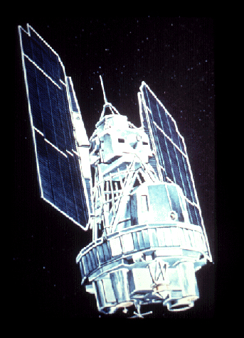
FIGURE 10: Artist’s view of Landsat 1.
Launched on July 23, 1972, Landsat 1, initially named ERTS (Earth Resources Technology Satellite), was the first satellite designed to study and to monitor the Earth’s surface, more specifically its landmasses. Figure 10 provides an artist’s view of the satellite. The sensors on Landsat 1 revolutionized remote sensing. They provided imagery in digital format and in multi-spectral form. It was the beginning of traditional aerial photography taken from planes for decades being replaced by digital imagery recorded from satellites.
Landsat 1’s two image sensor systems were the Return Beam Vidicon (RBV) built by the Radio Corporation of America (RCA) and the Multispectral Scanner System (MSS) built by General Electric. The RBV was supposed to be the primary instrument and the MSS, a highly experimental instrument, the secondary. However, the MSS imagery was found to be superior to the RBV imagery. In addition, the RBV instrument electronically interfered at times with the satellite’s altitude control functions; thus, it had to be shut down after recording only a few images. In comparison, the MSS acquired over 300,000 images before the operation of Landsat 1 was terminated in January 1978. The MSS sensor was the workhorse of the system and its success paved the way for the other satellites in the Landsat Program and imaging satellites developed by other countries and private companies.
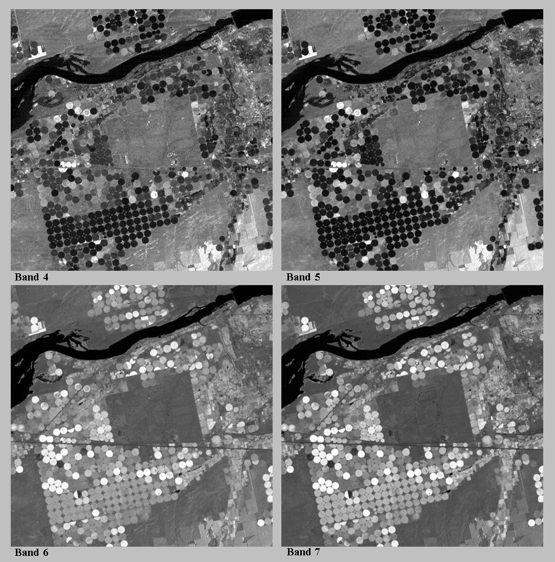
FIGURE 11: MSS bands showing center pivotal irrigation fields near the Columbia River in Oregon.
The MSS recorded data in four segments (spectral bands) of the electro-magnetic spectrum, namely in the green visible (0.5 to 0.6 µm), red visible (0.6 to 0.7 µm), near infrared (0.7 to 0.8 µm) and second near infrared (0.8 to 1.1 µm) segments of the spectrum (Figure 10). The four bands were numbered 4 through 7 since the RBV’s bands were identified as 1 through 3. The MSS scanned the Earth’s surface simultaneouslyin these four bands and from these scans created four digital images. A Landsat 1 scene covered a ground area of nearly 185 km (115 mi.) by 170 km (106 mi.) and had approximately 7,581,600 pixels (picture elements) per image band. A pixel was 56 m (183.7 ft) by 79 m (259.1 ft) in size, which is about 1.1 acres. Collectively, a data set of four bands had over 30,000,000 data values. The data values represented reflected energy from the Earth’s surface. With such a huge amount of data per one data set it was apparent that computers were going to be needed to process the images.
Figure 11 represents a subset of a MSS data set. It displays the four MSS spectral bands. The subset covers 1160 km2 (447.5 sq. mi.) and shows center pivotal irrigation fields along the Columbia River in Oregon.
MSS data were stored in an on-board recorder and downloaded electronically to one of three receiving stations. The stations were located in Alaska, California, and Maryland. Additional receiving stations were established in different sections of the World as the international community became interested in this new technology.
Dissemination of Landsat Data
NASA undertook an active program to disseminate Landsat data and train people and agencies on how to use this new technology. First, Landsat data sets and hardcopy image prints were easily available to anyone in the World and reasonably priced at $200 per data set (initially four 9 track computer tapes were needed for one data set) and $7 per hardcopy print (four prints were needed, one for each of the four bands) and $14 for a color composite print. Being so easily available Landsat imagery was like a gift being given by the United States to the World in order to study and plan the best use of our planet. For a time the largest purchasers of the data sets and images were the Soviet Union and the oil companies. Some less developed countries expressed concerns about foreign mining companies using the imagery to obtain knowledge about the possibility of certain minerals being available within a country’s borders, knowledge that a country might not possess. In other words, this new technology represented a new form of Western exploitation. These concerns disappeared once the countries found that they could afford the means to analyze the images themselves.
Second, to evaluate this new technology and to determine its potential applications, NASA funded 300 independent research projects. Nearly one-third of these projects were done by international researchers. A wide range of Earth science disciplines were represented in these projects.
Third, NASA established three training sites throughout the United States to introduce people at the state and local governmental levels on how to acquire, analyze, and use MSS data. The three sites were: Goddard Space Flight Center in Maryland, Stennis Space Center in Mississippi, and Ames Research Center in California. Training usually took one week of intensive work and involved a team of 4 to 8 people from a state or local governmental agency. In some cases training was provided for university/college faculty and Federal agencies. Training included various statistical procedures and computer hardware.
Finally, sizeable grants were given to the land grant colleges to obtain the necessary facilities and to prepare curricular materials based on this new technology. Each state has one land grant college and if a college received a grant, it was expected to provide training for people within its state.
The dissemination process included more than training of potential users. New computer hardware and software had to be prepared. Mainframe computers dominated in the 1960s and early 1970s. Basically these machines had 32-bit or higher word capacity that allowed them to do large numerical calculations. They were very fast and by the 1970s they had network capability that permitted terminals to link into them. In comparison the 32-bit microcomputer of today was in its infancy and had only an 8-bit word size that allowed it to handle only numbers between 0 and 255, not a machine on which to calculate large numbers. The primary output device on the mainframe computer was the high-speed line printer, designed mainly for printing numerical information. It was definitely not built for graphic output. However, due to some computer mapping programs, namely SYMAP, developed in the 1960s a way was discovered to make crude-looking graphics on line printers. Line printers could print 132 characters across a sheet of computer paper. To produce a reasonable size map or image several sheets of paper had to be printed and then taped together. This approach resulted in a rather large product that had to be placed on a wall from which one would have to stand several feet back in order to detect spatial patterns. Figure 12 illustrates a small section of such output. For Landsat output one printer character equaled one pixel. The elongated dimension of a printer character worked well with the 56 m by 79 m size of a Landsat pixel. A second output device existed at this time that was designed for vector graphics. It was the digital plotter that was produced mainly by the company Calcomp. It was a very slow output device that generally had to be run off-line from the mainframe. It was not designed for raster graphics associated with imagery output.
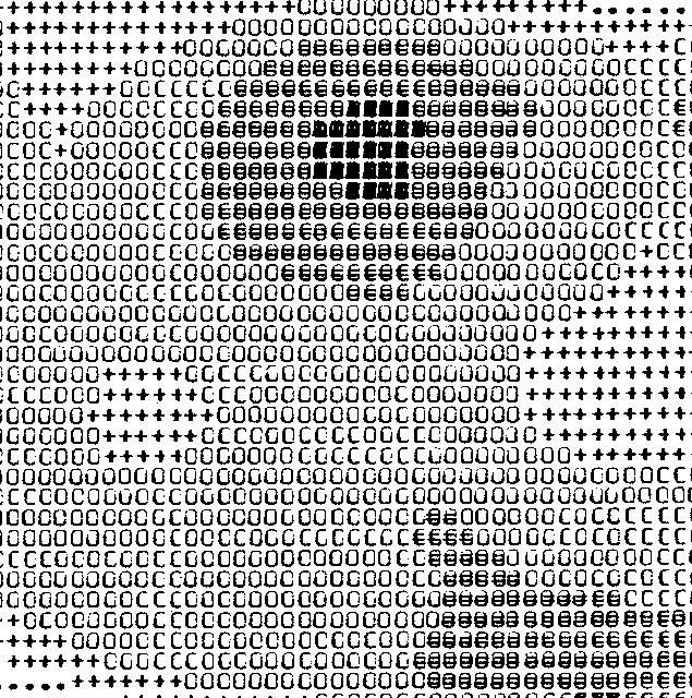
FIGURE 12: Line printer graphic output.
NASA was working with several companies to produce a fast raster image output device that would display images not only in black and white but also in color. One of the principal companies to develop such a device was COMTAL. The COMTAL device had a monitor that sat on a desk and in the desk was a large hardwired image processing board. This was the forerunner of today’s microcomputer monitors but microcomputers have a very small graphics microchip in place of the large hardwired board. Also, located on the desk was a terminal that was used to send messages to the mainframe and output would be sent back to the COMTAL monitor. However, mainframes were designed mainly to handle a variety of users who were doing minor numerical input and output work. A COMTAL device taxed the speed of a mainframe system that had a large number of other users. During this time minicomputers (16-bit word machines) were being manufactured that were produced to handle a single-type user rather than multiple-type users associated with mainframes. Three or four COMTALs could be linked to a dedicated minicomputer to create the desired image processing system to display and analyze Landsat imagery. Today this entire process can be handled on a microcomputer. Landsat played a key role in the implementation of the present microcomputers.
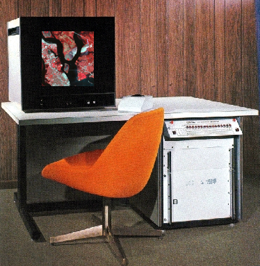
FIGURE 13: COMTAL image display unit.
In addition to hardware, software had to be prepared to handle the analysis of the multi band Landsat data sets. This software related mainly to image enhancement, geometric rectification, and information extraction. Image enhancement basically allowed changes to be made in the contrast and brightness of an image. Geometric rectification allowed images to be scaled and aligned with other raster data sets, namely topographic maps. Information extraction dealt with pulling out data from a spectral band(s). The information primarily sought related to land cover that is forests, open lands, wetlands, water bodies, and so forth. More specifically, the location and the amount of acreage for the different land covers were wanted. Two approaches were used to accomplish this task. The first approach, the supervised method, required developing spectral signatures from the four bands by statistically grouping the pixel band values for known land cover areas (Figures 14 and 15). For example, if four areas on the image were known to be of a particular type of forest cover, spectral signatures would be created for these four areas. This information would be used to identify any other pixels on the image with similar spectral signatures. Hopefully, all of the other pixels had the same type of forest cover. The second approach, the unsupervised method, would train the computer to seek image pixels with similar signatures and group them into unidentified spectral classes. An analyst would examine the classes and try to identify them with specific land covers. Once the spectral classes were developed under either the supervised or unsupervised approach, the statistics associated with the classes were sent through a classifier program. This program would classify the other pixels in an image by comparing their signatures to the spectral class signatures. A great amount of resources and energy was directed toward information extraction with some success. The main problem with this procedure was based on the land surface being more homogeneous than it is and spectral signatures relating to certain land covers.
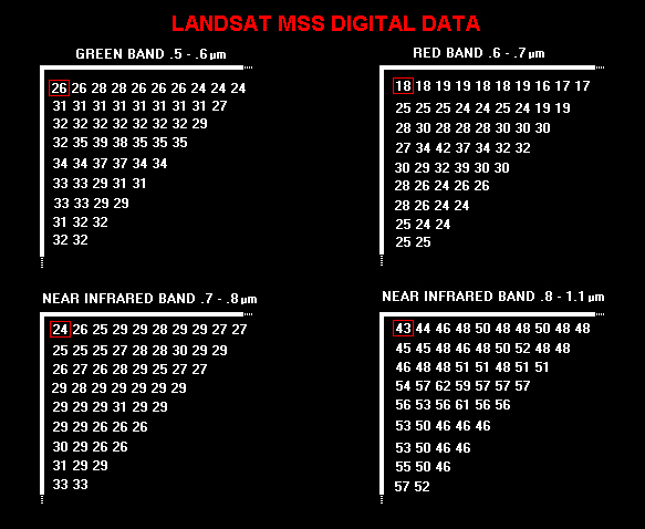
FIGURE 14: Sample of pixel values within a MSS data set. Values boxed in red relate to the spectral signature in Figure 15.
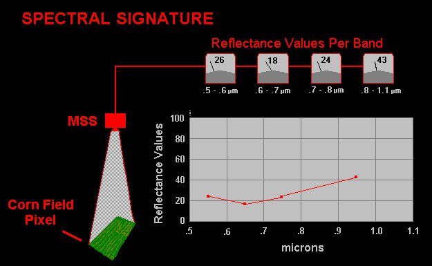
FIGURE 15: Sample spectral signature from one pixel in a corn field.
Landsats 2 and 3
Two other Landsats were put into operation during the 1970s. Landsat was launched on January 22, 1975 and remained operational for seven years until it was shut down on February 25, 1982. Like Landsat 1 it was considered experimental and maintained by NASA. It carried the same instruments as Landsat 1. Again the RBV instrument created problems and the MSS became the workhouse.
Landsat 3 was placed into orbit on March 5, 1978 and operated until September 7, 1983. It was still viewed as an experimental project and under the control of NASA until 1979. Because of the overall technical and scientific success of the Landsat Program, operational responsibility for the satellite was shifted from NASA, a research and development agency, to the National Oceanic and Atmospheric Administration (NOAA), the agency charged with maintaining the weather satellites.
Landsat 3 also had the RBV instrument but the instrument recorded only in one broad spectral band (green to near-infrared; 0.505-0.750 µm) rather than three bands like its predecessors. The ground resolution on this new instrument was 30 m (98.4 ft.) by 30 m (98.4 ft.). The instrument also had two parallel sensors with a certain amount of overlap.
A change was also made in the MSS. It still had four spectral bands but a fifth band that recorded emitted thermal energy was included. However, this band failed shortly after the satellite became operational.
Landsats 4 and 5
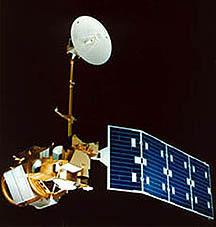
FIGURE 16: Artist’s view of Landsat 4.
During the 1980s some major changes occurred in the Landsat Program. These changes included: 1. a newly designed satellite and sensor system, 2. a new means for transferring data from the satellites, and 3. an attempt to move the program under the control of a private company.
On July 16, 1982, Landsat 4 was launched. It had its own satellite platform. Landsats 1-3 were built on platforms used for the Nimbus weather satellites. Compare Figures 10 and 16. The new platform carried the same MSS instrument found on previous Landsats but it did not carry the RBV instrument. A new sensor known as Thematic Mapper (TM) was added to the platform. The TM instrument scanned in seven spectral bands, namely the blue, green, red, near-infrared, mid-infrared (2 bands), and the thermal infrared portions of the electromagnetic spectrum. Except for the thermal infrared band, the bands had a ground resolution of 30 m (98.4 ft.) by 30 m (98.4 ft.). The ground resolution on the thermal infrared band was 120 m (393.6 ft.) by 120 m (393.6 ft.). Table 2 provides the basic characteristics of the TM bands. Figure 17 shows the seven over Charleston, South Carolina. Two color composite images are also provided. The true color composite is based on the three visible bands and is what a human eye would detect. The second composite is a false color arrangement. Due to the number of bands a large number of different false color composites can be created that allow various color patterns to be observed and information extracted.
Table 2: TM Bands
| Band No. | Wavelength Interval (µm) | SpectralResponse | Resolution (m) |
| 1 | 0.45 - 0.52 | Blue Green | 30 |
| 2 | 0.52 - 0.60 | Green | 30 |
| 3 | 0.63 - 0.69 | Red | 30 |
| 4 | 0.76 - 0.90 | Near IR | 30 |
| 5 | 1.55 - 1.75 | Mid-IR | 30 |
| 6 | 10.40 - 12.50 | Thermal IR | 120 |
| 7 | 2.08 - 2.35 | Mid-IR | 30 |
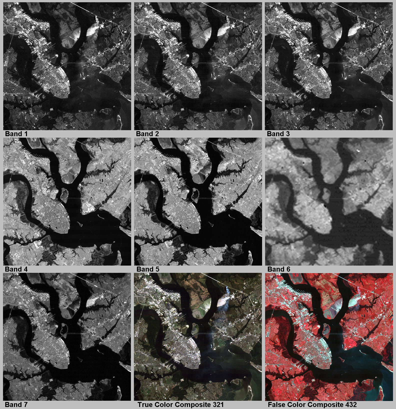
FIGURE 17: TM Bands.
Within a year after being launched, two of the solar panels on Landsat 4 stopped functioning as well as its two direct downlink transmitters. Thus, downloading imagery was not possible until a data relay satellite became operational. Imagery from Landsat 4 was transmitted to the relay satellite and the relay satellite downloaded the images to ground stations.
Landsat 5 was launched on March 1, 1984 with basically the same remote sensing configuration as Landsat 4. In 1987 its transmitter failed and it could no longer download international data to the U.S via the relay satellite. NASA engineers devised a way to handle this problem and Landsat 5 is still operational at the present time, 25 years after its designed life expectancy.
Privatization
In 1984 Congress passed the Land Remote Sensing Commercialization Act that privatized the Landsat Program. NOAA was charged to find a commercial vendor to take over the operation of the program. The Earth Observation Satellite Company (EOSAT), a partnership between Hughes Aircraft and RCA, was selected. EOSAT had a ten year contract to operate Landsats 4 and 5, exclusive rights to market Landsat data, and to build Landsats 6 and 7.
EOSAT raised image prices from $650 to $3700 to $4400 and restricted redistribution of images. These price increases resulted in many complaints from data users, users who had been cultivated by NASA dissemination efforts in the 1970s to use this new technology. Many of these users turned to lower resolution and lower priced images from meteorological satellites.
EOSAT did not maintain the necessary calibration of the Landsats 4 and 5 systems. In 1989, NOAA directed EOSAT to turn off the satellites. The data users were not willing to invest substantial amounts of resources into a program that had a questionable future. The program was saved by a strong protest from Congress, foreign and domestic data users, and the Vice President.
Also, in 1989 NOAA’s funding for transferring the Landsat Program ran out. Congress provided emergency funding for the rest of 1989 as well as 1990 and 1991. In 1992, new attempts were made to find on-going funding for the program. However, EOSAT had to cease processing Landsat data. In 1993 EOSAT was ready to launch its own satellite, Landsat 6, but the rocket failed to place the satellite in orbit. Although EOSAT tried for several years to continue operations by selling imagery from satellites operated by the Indian Remote Sensing Agency, it was apparent that privatization of the program was not successful.
Based on these issues the Land Remote Sensing Policy Act of 1992 was established. Under the act Landsat 7 was to be built and owned by the government. In 2001, Space Imaging, formerly EOSAT, returned operational control of Landsats 4 and 5 back to the government and relinquished all commercial rights to Landsat data that it had collected. This change allowed the prices on Landsat data to return to a more reasonable level and a better management of the satellites.
Landsats 6 and 7
As previously indicated Landsat 6, which was launched on October 5, 1993, failed to reach orbit due to a ruptured hydrazine manifold in the rocket. Fuel was not able to reach a kick motor device, resulting in not enough energy to place the satellite in orbit.
FIGURE 18: Artist’s view of Landsat 7.
Landsat 7 was successfully launched on April 15, 1999 (Figure 18) and began scanning the Earth using the ETM+ (Enhanced Thematic Mapper Plus) system. Landsat 7 is considered to be the most accurately calibrated Earth-observing satellite ever built. Its spectral band readings are extremely accurate when measured against the same ground readings. The ETM+ has the same seven bands found on Landsats 4 and 5 but it has an additional band that has a broad spectral range and a 15 m (49.2 ft.) by 15 m (49.2 ft.) ground resolution. Also, the ground resolution on Band 6, the thermal IR band, was increased from 120 m to 60 m. These changes along with its high accuracy level allow for better global change studies and large area mapping.
In May 2003 a hardware failure resulted in wedge-shaped spaces of missing data on either side of an image. A method has been developed to handle this problem.
The Landsat Program continues under the Landsat Data Continuity Mission. The next satellite is being built by General Dynamics Advanced Information Systems and is scheduled to be launched in 2012.
FINAL REMARKS
The CORONA (including the present KH satellites) and Landsat programs are the first and longest continuously operated satellite based remote sensing systems in their respective areas, CORONA in military reconnaissance and Landsat in Earth resource monitoring. Both programs established many of the procedures and systems being used on the wide variety of satellites circling the Earth today remotely sensing the planet.
REFERENCES:
Clarke, K. 1999, Project Corona, sponsored by the National Science Foundation. Santa Barbara. http://www.geog.ucsb.edu/~kclarke/Corona/Corona.html.
Jensen, J.R., 2000, Remote Sensing of the Environment: An Earth Resource Perspective, Upper Saddle River, New Jersey: Prentice Hall, 656pp.
Power, F.G. Jr., 1997, “Foreword: From the U-2 to Corona.” CORONA: Between the Sun and the Earth: The First NRO Reconnaissance Eye in Space, R.A. McDonald Ed., Bethesda: American Society for Photogrammetry & Remote Sensing, vii-ix.
Ruffner. K. C. 1995, CORONA: America’s First Satellite Program, Washington D.C.: Central Intelligence Agency, 360 pp.
The Landsat Program, Ames Research Center. http://geo.arc.nasa.gov/sge/landsat/daccess.html
The Landsat 7 Gateway, Goddard Space Flight Center. http://landsat.gsfc.nasa.gov/