|
|
|
|
THE DRY MONSOON
OF THE DECCAN PLATEAU, INDIA
COPYRIGHT © 2001 Paul R. Baumann
INTRODUCTION:
India’s summer monsoon represents one of the most dramatic seasonal weather changes in the world. Its impact must not only be measured in terms of its meteorological occurrences but also how it affects the lives of nearly one-fifth of the world’s people. “The fate of India is bound head and tail to the course of the monsoon,” says monsoon expert David Stephenson, of Meteo-France, a research institute in Toulouse, France. “If the rains come too late, farmers will sow few or no seeds, fearing a drought. If there is a lack of continued showers or breaks in the rain, plant seedlings may not survive. If the rains are too hard, young plants and seedlings can be washed away. All these factors can greatly increase the price or decrease the availability of food in India.”
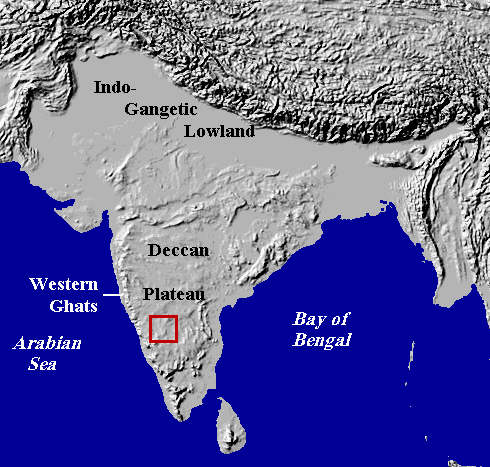
Figure 1: Subcontinent and Study Area (in red).
The word “monsoon” is generally associated with heavy rain, which is often a mid-latitude perception of a monsoonal condition. A monsoon in the low-latitude sections of the world refers to a seasonal shift in wind direction. The word is derived from the Arabic term “mausim”, meaning season. Monsoonal winds typically cause drastic changes in precipitation and temperature patterns. A monsoon may be associated with dry weather as well as wet weather, since the “wet” monsoon phase of warm, moist air is seasonally replaced by a “dry” monsoon of cool, dry air. Even during the wet monsoon season, not all sections of India and the remainder of the Subcontinent receive large amounts of rain. Major sections of the region receive light to moderate rainfall but the amount received is considerably more than obtained during the dry monsoon period. One of these sections is the Deccan Plateau of south India where various means have been developed, including the building of large reservoirs, to capture and hold water for the dry monsoon period.
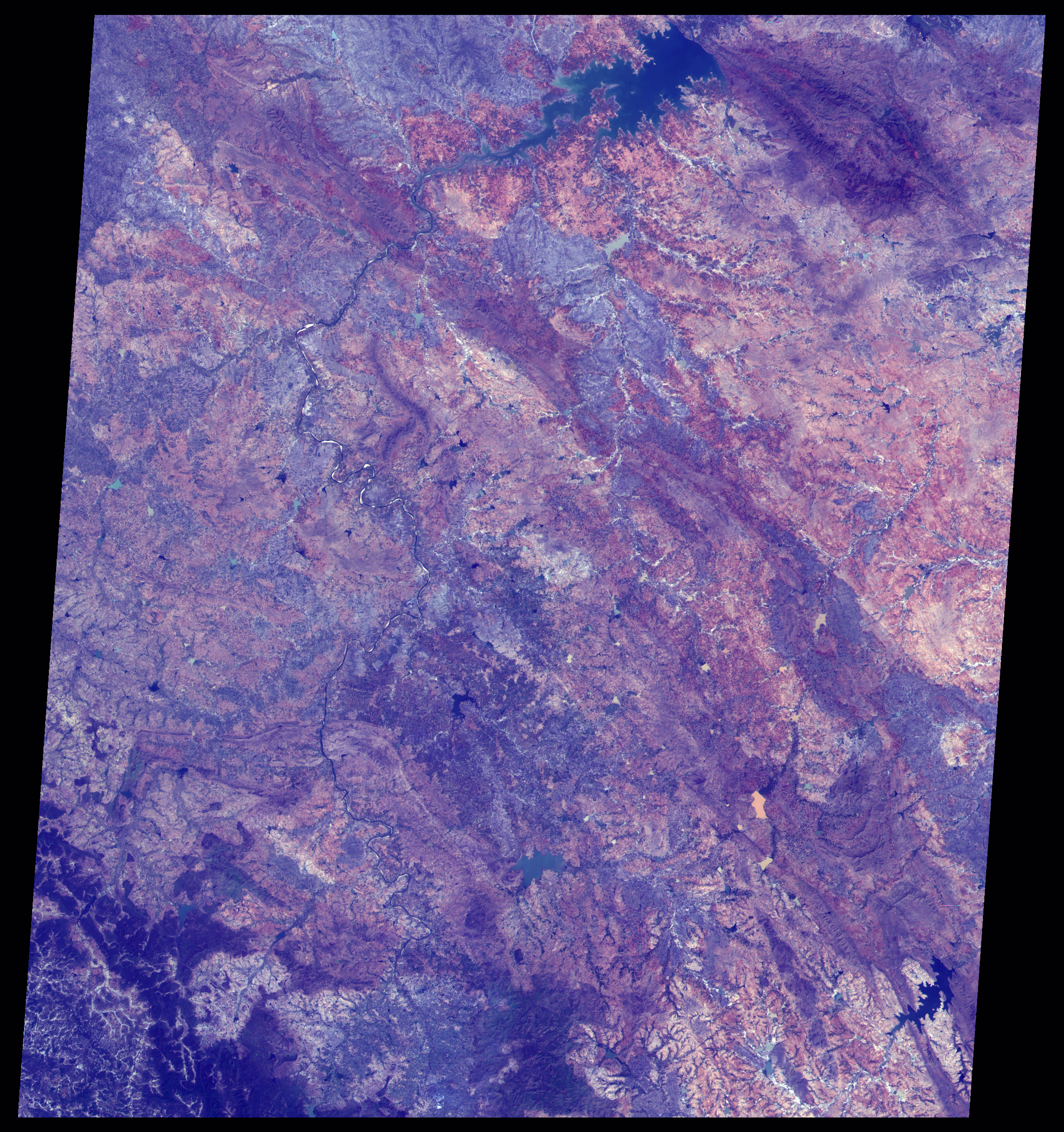
Figure 2: True Color Image of Study Area.
Click on image to view full scale image.
In general, this instructional module examines the climatic and water issues of the Deccan Plateau. More specifically, it uses a satellite multi-spectral data set to measure the water conditions of the Tungabhadra Reservoir, one of the principal reservoirs on the plateau. The data set was acquired on February 9, 1993, by the Linear Self Scanning Sensor (LISS-I) aboard India’s IRS-1B satellite. Figure 1 identifies the location of the study area on the Subcontinent and Figure 2 shows the area encompassed by the data set.
BACKGROUND:
MONSOON CLIMATE
The summer monsoon patterns of India and the other sections of the Subcontinent are the result of the interaction of several climatic controls. The first of these controls is sun and latitude. Since the Earth’s axis is tilted in relationship to the Sun’s axis, the intense, vertical rays from the Sun vary in location throughout the year from the Tropic of Cancer (23 ˝ degrees N.) to the Tropic of Capricorn (23 ˝ degrees S.). This shift in the vertical rays not only results in seasonal temperature differences on the Earth’s surface but also brings about the north-south migration of major pressure zones such as the Equatorial Low and Subtropical Highs and wind flows such as the Tropical Easterlies and Westerlies.
The second climatic control relates to land and water distribution. Land and water surfaces are cooled and warmed at different rates based on the amount of sun radiation being received. Thus, it is important to understand the geographic distribution of such surfaces. In examining a world map, one can see that the Pacific and Atlantic Oceans extend as major water masses from the Arctic to the Antarctic. The same is true for the land masses of the Americas and Europe/Africa. These patterns create a duplicate set of pressure and wind zones on each side of the Equator that migrate back and forth with the seasons. However, these patterns change when dealing with the Indian Ocean and Asia. No longer does a continuous water or land surface exist between the Arctic and Antarctic regions, but instead, a water surface occurs basically in the Southern Hemisphere and a land surface in the Northern Hemisphere. This difference changes the pattern of pressure and wind zones from those found in other areas of the world. A second land-water distribution pattern to note is the lack of any large land surface at the Equator in this section of the world. In the Americas one finds a large land mass, namely the Amazon Basin, at the Equator and in Africa the Congo (Zarie) Basin. A large land mass at the Equator results in the development of a strong Equatorial Low Pressure Cell. Such a cell does not exist over the Indian Ocean during the summer period in the Southern Hemisphere. During the summer period in the Northern Hemisphere a cell does develop but not over the Equator. It occurs farther north, mainly over the Indo-Gangetic lowland of Pakistan and India. These land-water distribution patterns play a key role in setting the stage for the development of the summer monsoon over the Subcontinent.
A semi-permanent Subtropical High Pressure Cell exists off the west coast of Australia. During the summer period in the Southern Hemisphere, Tropical Easterlies flow from the northern portions of this cell across the Southern Indian Ocean picking up moisture. These moist winds are eventually heading toward an Equatorial Low pressure cell over central Africa, south of the Equator. During the summer period in the Northern Hemisphere this African Equatorial Low pressure cell moves north of the Equator. It is following the vertical rays from the the sun. The moist Tropical Easterlies winds from the Australian Subtropical High Pressure Cell, which has now shifted to the center of the Indian Ocean, flow initially toward the African Equatorial Low Pressure cell but they must now travel over the Equator, which introduces Coriolis force. According to this force, fluid items in the Northern Hemisphere move to the right of their point of origin and to the left in the Southern Hemisphere. Starting in the Southern Hemisphere the moist Tropical Easterlies are moving to the left of the Subtropical High Pressure Cell but once they cross the Equator, they change directions and move away from Africa. If one was standing at the southern end of the Arabian Peninsula at this period, one would encounter clear skies above but could observe the clouds over the Arabian Sea flowing from west to east toward India. These winds are moving toward another Equatorial Low pressure cell, one that has developed over the Indo-Gangetic lowland. See Figure 3.
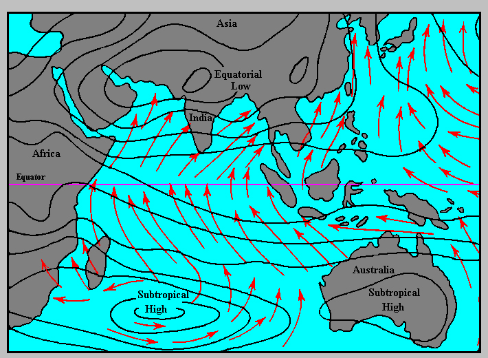
Figure 3: Pressure Cells and Tropical Easterlies over the Indian Ocean in July.
Since the Tropical Easterlies have crossed several thousand miles of warm water, they arrive on the west side of India and Pakistan with large amounts of moisture in the air. However, the land is warmer than the water, which would typically increase the capacity of the air to hold moisture and decrease the likelihood of any precipitation. At this point other climatic controls enter the picture. The first centers on topographic barriers. Along the west coast of India is the Western Ghats, which form the western edge of the Deccan Plateau. They rise abruptly from the coastal plain and reach heights between 4,000 and 8,000 feet (1219 and 2438m) and then gently slope down to the Deccan Plateau. When the moist, monsoon air encounters this topographic barrier, the air is forced to rise, and in the process, cools. When the air cools, its ability to hold moisture decreases and the chance for precipitation increases. This condition creates what is called “orographic precipitation.” In this particular situation, a great amount of precipitation occurs with totals reaching between 100 and 200 inches (254 and 508 cm.) within a 4 or 5 month period. Check the west coast of India on Figure 4. The eastern Himalayas experience even an greater amount of orographic precipitation. It is the Western Ghats and the Himalayas that people generally associate with the monsoon since these areas receive such great amounts of precipitation during a particular season of the year.
Figure 4: Geographic Distribution of Precipitation.
Once the Tropical Easterlies drop a substantial amount
of their moisture by crossing over the Western Ghats, they descend down onto the
Deccan Plateau. Here rainfall decreases significantly but people greatly enjoy the
arrival of the monsoon winds. They have endured hot, dry stagnant air for several
months and appreciate the flow of air. However, the hot air over the plateau
pulls the monsoon winds into a convectional condition forcing the air to rise
and cool. This process causes convectional storms (thunderstorms) and represents
the other climatic control to produce rain from the Tropical Easterlies or
monsoon winds. Eventually the winds cross the plateau and enter the Bay
of Bengal where their moisture content is replenished. They now move toward
the Himalayas and the Indo-Gangetic lowland where the Equatorial Low
Pressure awaits them. A combination of orographic and convectional conditions
brings about large amounts of precipitation during the monsoon season.
DECCAN PLATEAU
The Deccan Plateau is a large region that covers most of south central India. It can be divided into two major sections, the North Deccan and the South Deccan regions. Although the two regions are similar in elevation, climate, and natural vegetation, the South Deccan has no major lava formations to enrich the soil. Red-loam or sandy loam soils usually overlie the granites and metamorphic rocks resulting in less fertile and less moisture retentive soils than found in the North Deccan region. This instructional module deals with only the South Deccan, an area of 127,700 square miles (330,743 sq. km), which lies mainly in the state of Karnataka (formerly Mysore) and Andhra Pradesh.
Figure 5: Precipitation Profile from the Western Ghats to the Deccan Plateau.
The average elevation is 1,000 to 2,000 feet (305 and 610m) above sea level along the northern sections of the region and 2,000 to 3,000 feet (610 and 915m) in the southern section. The region slopes generally eastward allowing the drainage to flow toward the Bay of Bengal. Water in the rivers fluctuates considerably during the monsoon and the dry seasons. Their only source of water is the monsoon rains unlike the rivers flowing out of the Himalayas that have year-round moisture from snow packs in the high mountains. In the winter or dry season many of the rivers throughout the South Deccan become almost dry and are useless for irrigation. Also, some of the rivers flow through well-incised valleys, allowing little space for a flood plain and making it nearly impossible to direct water for irrigation onto the adjoining uplands.
The climate is generally semi-arid with less than 35 inches (89 cm.) of rainfall. Ironically, the Western Ghats are only 30 to 40 miles (48 to 64 km) away with annual precipitations exceeding 100 inches (254 cm.). Figure 5 clearly illustrates this situation by showing the precipitation patterns for four weather stations. The first station is located immediately on the coast and is only 203 feet (62m) above sea level. The second station falls in the heart of the Western Ghats and is over 4,000 feet (1220m) in elevation. The third station is on the eastern edge of the Western Ghats. The larger rivers on the Deccan Plateau get most of their water from regions typical of the third station but the water is mainly seasonal. The water from the second station moves rapidly down the western slopes of the Western Ghats and returns quickly to the Arabian Sea. The last station is representative of the driest sections of the South Deccan. The first two stations derive most of their precipitation between June and September from the southwest monsoons. The last two stations also receive moisture from the southwest monsoons but they do get some moisture between October and November from what is referred to as the “retreating monsoon.”
Figure 6: Water Balance Budget at Honavar.
Figures 6 and 7 provide the water balance budgets for two weather stations. The first station, Honavar, is located on the coast and the second station, Bellary, is situated in the center of the South Deccan. Figure 4 shows the location of the two stations. The water balance budget compares the rainfall distribution throughout the year to the potential evapotranspiration distribution. In this situation evapotranspiration deals with the amount of moisture removed mainly from the soil due to evaporation. Honavar starts the year with the potential evapotranspiration rate being higher than the rainfall. To make up the difference between the potential evapotranspiration level and the actual rainfall, moisture is taken from the soil. Somewhere between May and June the precipitation level exceeds the potential evapotranspiration level and the soil is recharged with moisture. From June to mid-October, the amount of precipitation continues to exceed the potential evapo-transpiration level. The soil at this point is saturated and cannot absorb any more moisture. This water surplus becomes surface water, which runs off into the sea. In November the potential evapotranspiration rate surpasses the rainfall level again but the soil has enough moisture to sustain the growth of vegetation until it is recharged with the coming of the summer monsoon. Thus, one is observing the annual cycle of life associated with the monsoon. In the case of Bellary, the potential evapotranspiration level greatly exceeds the amount of precipitation throughout the entire year. No moisture surplus ever occurs in the soil. The phrase “dry as a bone” reflects the moisture condition at Bellary and surrounding region. India’s challenge is how to get the water surplus at Honavar to Bellary, a good example of the geography of water.
Figure 7: Water Balance Budget at Bellary.
Due to the constant water storage in the South Deccan, numerous attempts have been made to capture water during the so-called dry season to be used during the wet season. Many farmers and communities construct small reservoirs, known as tanks. Some tanks have existed for over a thousand years. Tanks range from shallow ponds dug to catch rainwater to dams across small streams. They might cover many square miles or less than an acre. Tanks are scattered across the South Deccan landscape. In Figure 8, a Landsat false-color image of a small section of the South Deccan landscape, hundreds of tanks ranging from black to light blue in color can be observed. Animals use the water in the tanks; people wash their clothes and vegetables in them; refuse is dumped in them; and fish are obtained from them. Tanks provide the only water for domestic use. By the end of the dry season the tanks have shrunk to a fraction of their normal size.
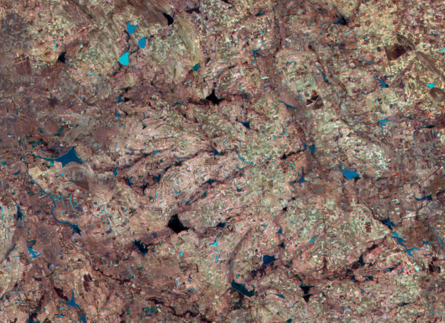
Figure 8: False Color Landsat Image Showing Tanks.
In addition to tanks, median and large reservoirs have been constructed. Such reservoirs have been built by either states or the national government. Figure 9 is a photograph taken from one of the Space Shuttles over the South Deccan. A large reservoir along with several medium size reservoirs can be detected. Also, the brownness of the bare landscape can be observed in comparison to the green of the Western Ghats. Note the amount of sediment washing into the Arabian Sea from the Western Ghats.
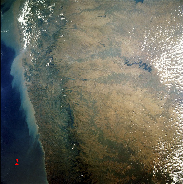
Figure 9: Space Shuttle Image of the South Deccan and Western Ghats.
TUNGABHADRA RESERVOIR
Several large reservoirs have been built in the South Deccan, one of which is the Tungabhadra Reservoir. This instructional module focuses in on this reservoir and examines some of the problems encountered by having a large water body in a dry region. The remote sensing component of this modules deals with: 1) exploring synoptically the reservoir and surrounding region and 2) measuring the surface area of this reservoir during the dry season.
The Tungabhadra River derives its name from the Tunga River, about 91.6 miles (147 km) long and the Bhadra River, about 110.9 miles (178 km) long, which rise in the Western Ghats. The two rivers merge near Shimoga. From this point the Tungabhadra runs for about 330 miles (531 km) before joining with the Krishna River at Sangamaleshwaram in the state of Andhra Pradesh. More specifically, it runs for 237 miles (382 km) in the state of Karnataka, and then forms the boundary between Karnataka and Andhra Pradesh for 36 miles (58 km). Finally it runs for the next 57 miles (91 km) in Andhra Pradesh. The river’s total catchment area is 26,856 sq. miles (69,552 sq. km) up to the point of flowing into the Krishna. It is a perennial river, which chiefly receives its water from the Southwest Monsoon; however, in the dry season its flow dwindles considerably.
Endemic levels of famine throughout the region attracted the attention of the British engineers as early as 1860. To relieve the intensity of famine a proposal was made to utilize the waters of Tungabhadra through a storage reservoir and a system of canals to provide irrigation for the lands. Sir Arthur Cotton originally put forth the Tungabhadra Project in 1860.
However, the Prince of Berar, on the left side of the river, and "Sir Arthur Hope" Governor of Madras, on the right side, did not formally inaugurate the Tungabhadra Project until February 28, 1945. The proposed site selected for the dam and reservoir was at the section of the river that formed the boundary between the native state of Hyderabad (the Nizam’s Dominions) and the province of Madras, under more direct British control. The catchment area of 10,880 sq. miles (28,177 sq. km) for the reservoir resided in the state of Hyderabad, now Karnataka; most of the irrigation water from the reservoir was going to the province of Madras, now the state of Andhra Pradesh.
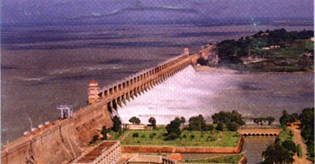
Figure 10: Tungabhadra Dam
Between 1901 and 1945, Hyderabad refused to cooperate, arguing that fifty-four square miles (140 sq. km.) of its prime farmland would be below the proposed lake. After an agreement was finally reached in 1944, progress on the actual building of the dam continued to be a problem because both sides wanted to control construction. Finally, the dam was built to a common design by separate teams working from either bank. See Figure 10. By October 1953, the dam was completed substantially enabling the storage of water in the reservoir up to 1613.00 ft. Acquisition of lands and villages and rehabilitation of persons displaced from the water spread area up to the 1630ft contour had been completed by September 1953. About 90 villages and 54,452 people were affected. After India gained its independence, state boundaries were redrawn resulting in the dam being completely in the now state of Karnataka. Disputes continue between Karnataka and Andhra Pradesh over the feeder irrigation canals, which cross back and forth over the boundaries between the two states. The building and operation of this reservoir represents a good case study in political geography.
Water management of a reservoir requires having a fairly accurate assessment of the reservoir’s storage capacity. Siltation is a major storage capacity problem facing all reservoirs. In 1953, when the Tungabhadra Reservoir was first impounded with water, its capacity was nearly 133.0 BCft (billon cubic feet). In the initial planning stages it was envisioned that the annual silt deposition in the reservoir would range between 420 and 430 MCft (million cubic feet), with about 25 percent of the silt flushing through the reservoir. In order to assess the rate of siltation in the reservoir, hydrographic surveys have been conducted since 1963. The initial survey in 1953 was done topographically. Table 1 shows the capacity figures recorded for certain years. For the first 10 years, the annual rate of siltation was on the order of 1.78 BCft. During the last 12 years, 1981-1993, the rate of siltation has decreased to 0.41 BCft per year. For the 40 years between 1953 and 1993 the siltation rate averages about 0.52 BCft or 520 MCft per year. This rate is about 100 MCft more than the original estimate of between 420 and 430 MCft and does not include the approximate flushing level of 25 percent. In other words, the Tungabhadra Reservoir has lost 21 BCft or about 16 percent of its useful storage. This decrease in capacity has reduced the amount of irrigation water from 212 BCft to 187 BCft per year. These figures do not take into account evaporation losses. Dredging the reservoir has been studied but the cost involved in removing the silt from the reservoir and transporting it to a safe area makes dredging not economically feasible.
TABLE 1: CAPACITY FOR TUNGABHADRA RESERVOIR
| Year of Survey |
Capacity at FRL (1633 ft.) BCft (M.Cum) |
| 1953 | 132.473 (3751.17) |
| 1963 | 114.660 (3246.79) |
| 1972 | 121.080 (3428.60) |
| 1978 | 117.696 (3332.75) |
| 1981 | 115.681 (3275.68) |
| 1985 | 111.832 (3166.74) |
| 1993 | 111.508 (3157.53) |
| FRL = Full Reservoir Level; BCft = One billion cubic feet |
| M.Cum = Million cubic meters |
Why do such high levels of siltation occur in the Tungabhadra Reservoir? First, water bodies in dry regions generally have higher rates of siltation than similar water bodies in humid regions. In dry regions the land has less vegetation coverage, and therefore, is more susceptible to erosion when rain does occur. The Tungabhadra Basin, as previously indicated, is a semiarid region. Second, streams or rivers that vacillate greatly with respect to water level often have sediment build-up in the river bed during the dry season, which is washed down the river during the wet season. The monsoons provide the stage for this vacillation in water levels in the Tungabhadra River and other streams within the basin. Note in Figure 11 all of the sediment build-up along the Tungabhadra River during the dry season. Third, the numerous tanks throughout the basin reduce the amount of water available to flow into the reservoir, creating lower water levels in the river during the dry season and more sediment build-up along the river. It is estimated that between 25,000 and 30,000 tanks exist in the basin. At the same time the tanks collect sediment that would normally flow into the reservoir. Fourth, industrial pollution has contributed to the siltation problems of the reservoir. For example, the pulp based industries on the Tungabhadra have impaired the groundwater recharge within the basin by developing large-scale cultivation of pulpwood species, like Eucalyptus. Many other siltation issues impact the reservoir. Unless some major steps are taken to rectify these issues the reservoir has probably another 50 years of effective use.
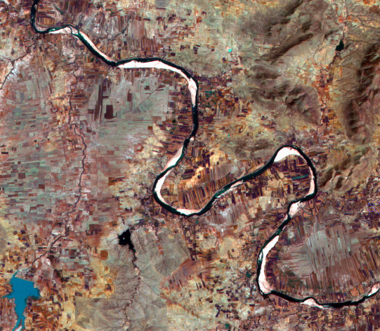
Figure 11: Sediment build-up along the Tungabhadra River.
ANALYSIS:
DATA SET
Two data sets are available with this instructional module. However, the work outlined below is based on only using one of these data sets. The second data set is made available for one to examine certain areas in more detail. The two data sets were recorded at the same time on February 9, 1993, using sensors aboad India’s IRS-1B satellite. The primary data set is 2500 scan lines and 2350 picture elements in size and has a picture element resolution of 72.5 x 72.5 meters. The secondary data set is also 2500 scan lines and 2350 picture elements in size but has a picture element resolution of 36.25 x 36.25 meters. Although the primary data set does not have the spatial detail which the secondary data set has, it does provide full coverage of the Tungabhadra Reservoir and greater coverage of the South Deccan region than the secondary data set. The secondary data set does provide more detail but for only a certain portion of the area covered by the primary data set.
The first two IRS (Indian Remote Sensing Satellite) satellites, IRS-1A (March, 1988) and IRS-1B (August, 1991) were launched by Russian Vostok boosters from the Baikonur Cosmodrome, Russia. IRS-1A stopped functioning in 1992, while IRS-1B continued to operate through 1999. The two spacecrafts each operated three Linear Imaging Self-Scanning (LISS) remote sensing instruments and each instrument recorded in four spectral bands. The spectral range for the four bands are provided in Table 2. The LISS-I covers a swath of 148 km with a resolution of 72.5 m while the LISS-IIA and LISS-IIB instruments exhibit a narrower field of view (74-km swath) but are aligned to provide a composite 145-km swath with a 3-km overlap and a resolution of 36.25 m.
TABLE 2: BAND SPECTRIAL RANGES
| Band 1 | 0.45-0.52 µm | Visible (Blue) |
| Band 2 | 0.52-0.59 µm | Visible (Green) |
| Band 3 | 0.62-0.68 µm | Visible (Red) |
| Band 4 | 0.77-0.86 µm | Near Infrared |
IRS-1C was successfully launched on December 28, 1995, while IRS-1D was placed in orbit by India's PSLV spacecraft on September 29, 1997, from Sriharikota, India. These satellites provide better spatial detail and different spectral bands than the first two satellites.
India started development of its Indian Remote Sensing
Satellite program to support its national economy in the areas of "agriculture, water
resources, forestry and ecology, geology, watersheds, marine fisheries and coastal
management". The Indian Remote Sensing satellites are the foundation of the
National Natural Resources Management System (NNRMS), for which the
Department of Space (DOS) is the principal agency, providing operational
remote sensing data services. Data from the IRS satellites is received and
disseminated by several countries all over the world. With the advent of
high-resolution satellites new applications in the areas of urban sprawl,
infrastructure planning and other large scale applications for mapping have
been initiated.
SYNOPTIC VIEW
One of the best tools available to geographers in studying a region is to obtain an overall or synoptic view of the area. A remotely sensed image provides such a view. Kevin P. Corbley, a freelance writer specializing in remote sensing, GIS, and Global Positioning System (GPS) technology, conveyed the following occurrence in the June 1997 issue of Geo Info Systems. This occurrence illustrates the importance of remote sensing and the synoptic view in addressing human needs. It also deals directly with the region being studied in this instructional module.
"On a sunny afternoon in October 1996, a small group of farmers wearing traditional village dress arrived unannounced at the Indian Space Research Organization (ISRO) in Bangalore, India. ‘We need water,’ they told the bewildered security personnel at the front gate. The security crew thought the farmers, who had traveled some 300 kilometers from the Bellary District north of Bangalore, had reached the wrong destination and were about to turn them away. The farmers repeated their request, asking to speak with scientists who use ‘instruments in space’ to find underground water that might save their farms from drought.
“Word of their plight reached ISRO managers inside, and a team of remote sensing geologists was immediately assembled to use imagery from the Indian Remote Sensing (IRS-1C) satellite to find drilling sites for new wells. The geologists analyzed multispectral images from the satellite’s Linear Imaging and Self-Scanning Sensor 3 (LISS-3) sensor to decipher the complex geology around the village. Multispectral signatures of various rock layers helped them pinpoint formations known to be associated with groundwater.
“The farmers gladly collected ground-truth information to support the project. Within the week, ISRO - with help from IN-RIMT (Bangalore), a private consulting company - had identified potential drilling sites that ultimately provided water for the villagers. Such grassroots requests for remote sensing information are not uncommon in India, according to Mathewkutty Sebastian, an ISRO earth observation systems scientist. ISRO representatives take great satisfaction in relating the story of the Bellary farmers because, as Sebastian put it, ‘The satellite was designed with them in mind.’”
One of the best ways to obtain a synoptic view using remotely sensed imagery is to create color composites of full data sets and then pan through the composites observing patterns on the Earth's surface and the interrelationship between features on the surface. The software package, EarthScenes, is used throughout this module and easily allows one to develop color composites and pan through these color images. Assigning three spectral bands to the three basic colors - red, green, and blue - creates a color composite. If the same band is used for each color, a black and white image is produced. A “true color composite” occurs when the red visible band is assigned the red color, the green visible band the green color, and the blue visible band the blue color. This is how the human eye would see the surface. All other composites are called “false color composites.” In making a true color composite of the data set being used in this module, the landscape will seem blue and red in color with little emphasis on green, which is an indication of how dry the surface is. Figure 2 is a true color composite.
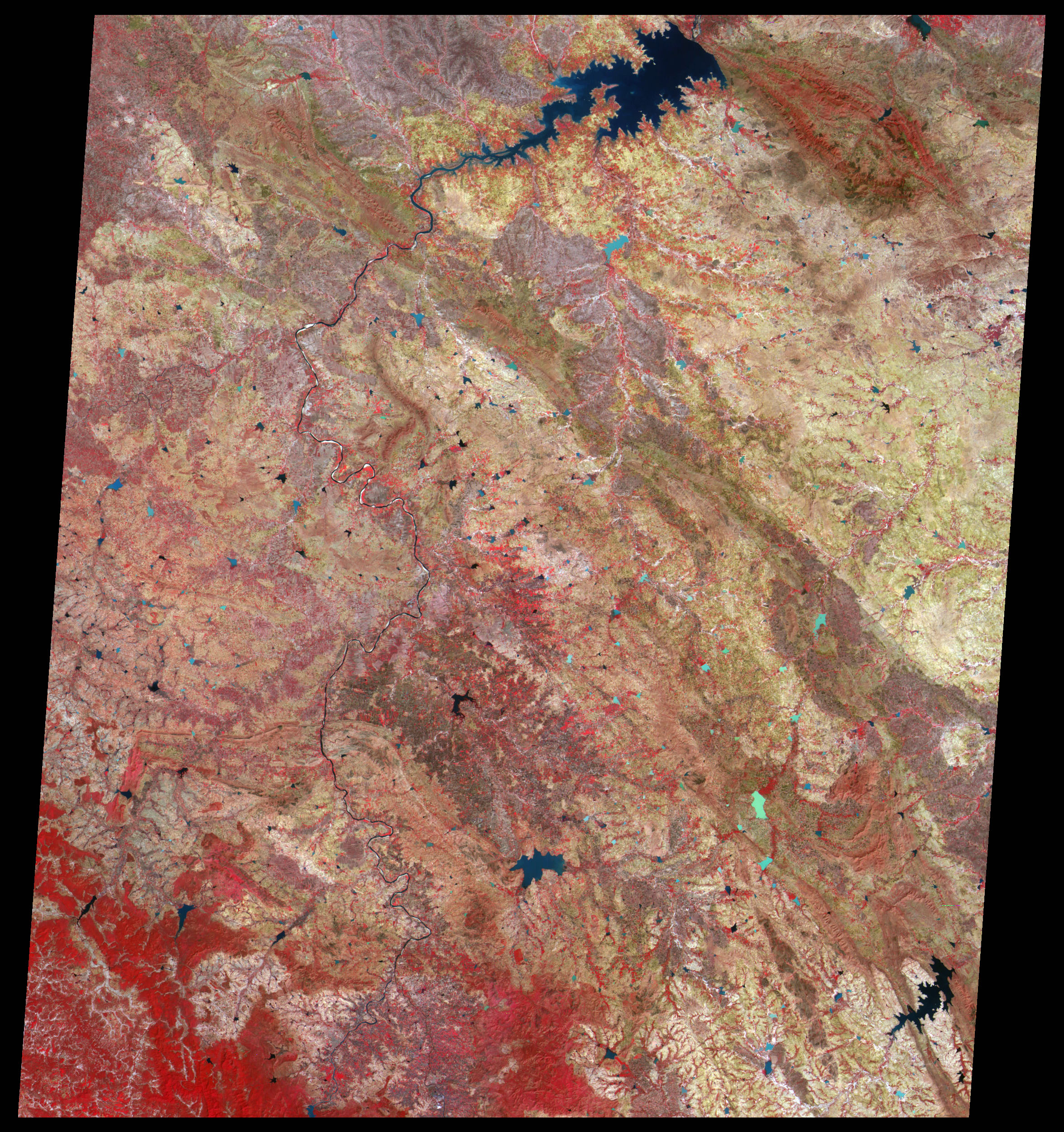
Figure 12: False Color Composite of Study Area
Click on image to view full scale image.
Figure 12 is one of several different combinations of bands that can be used to create a false color composite. In this case the infrared band was assigned to the red color, the red visible band to the green color, and the green visible band to the blue color. The body of water in the northeast section of the image is the Tungabhadra Reservoir. The Tunga River, which originates in the Western Ghats, runs through the middle of the image. In the extreme southwestern portion of the image, the eastern edge of the Western Ghats can be seen in a dark red color indicating lush vegetation coverage. Agricultural field patterns can be easily identified. Fields with bare soil are in green, and vegetated fields are in shades of red. Intermediate stages of vegetation growth are shades of yellow and gray. Tanks are in various shades of blue. Reddish-brown hills, more than 1000 ft. (305m) above the plateau surface, are aligned northwest-southeast. The Tungabhadra River originally cut through a gorge in one of these hill alignments. This gorge became the site for the construction of the Tungabhadra Dam. The front of the Tungabhadra Reservoir spreads out along the western side of these hills. Although Figure 12 provides a nice comprehensive picture of this particular composite image, much more detailed information can be observed on the image by using EarthScenes’s “Color composite pan and roam” function. It is best to use the “pan and roam” function on any large image, which exceeds the size of the monitor screen. The combination of the “color composite” and “pan and room” functions provides one with a good synoptic viewing tool, and thereby, the ability to analyze the geographic interrelationships of a region.
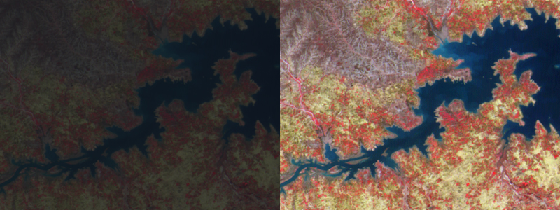
Figure 13: Regular bands versus stretched bands.
The reflectance levels of a spectral band are recorded as numerical values generally ranging between “0” and “255.” A “0” value indicates a low reflectance and appears black on a gray scale image; whereas, a “255” value is a high reflectance condition and shows as white. Most spectral bands do not record reflectance values covering this full potential range. The reflectance values are frequently clustered in a certain section(s) of the full range. This condition results in a limited portion of the gray scale being used and produces a dull looking image. To overcome this problem, the reflectance values for a band can be stretched over the full potential data range, which in turn, produces an image based on the full gray scale. This process is called “Contrast Stretch.” EarthScenes provides this function. Contrast stretched bands generally produce better-looking color composite images than the regular bands. Figure 13 compares a color composite of three regular bands with the same three bands after being stretched. The combination of bands used to form Figure 12 is the same combination used in Figure 13. It is apparent from Figure 13 that the bands used in making Figure 12 were stretched.
To stretch an image, certain statistical parameters about the image must first be obtained. In EarthScenes, the “Create a histogram” function accomplishes this task. This function only has to run once for a particular image. Next one might wish to plot the results of the histogram to receive some visible idea about the distribution of the data. “Plot the histogram” function in EarthScenes produces a graph showing the distribution of the data for an image. Rather than using the full potential range of “0” to “255,” EarthScenes uses a range from “1” to “250.” Table 3 shows for each of the four bands the original minimum and maximum values, the mean score, the minimum and maximum values used to stretch a band, and the mean score of a stretched band. The author of the module selected the minimum and maximum values used to stretch the bands shown in Table 2. Another person might select different values. The mean scores of the unaltered bands are located at the low end of the full potential range. The mean scores of the stretched bands are more centered in the full potential range. In the stretching process the new minimum and maximum values are assigned the values of “1” and “250,” respectively, by EarthScenes and all of the values in between are given new values proportional to this scale. All values below the minimum are assigned the value of “1” and values above the maximum are given the value of “250.” For example, the original minimum and maximum values for Band 1 are “1” and “68” and the minimum and maximum values used to stretch the band are “31” and “68.” In examining either Figure 2 or Figure 12, one will note a large black area around the edge of both images. Although this black area is not part of the image, it is part of the data file associated with the image. All the picture elements in this black area have been given the value of “1.” This situation distorts the true minimum value of the image, which is “31.” The “Plot the histogram” function assists in finding the true minimum value. In stretching the image, all values of “31” and below became “1” and all values of “68” and above became “250.” One can stretch the data in many various ways to bring out new information on an image. Thus, the contrast stretch function introduces a third tool, along with the color composite and pan and roam tools, for a remote sensing analyst to use in a synoptic analysis.
TABLE 3: ORIGINAL AND STRETCHED BAND PARAMETERS
| Band No. | Original |
Original |
Mean |
Stretched |
Stretched |
New Mean |
| 1 | 1 | 68 | 38.9 | 31 | 68 | 80.5 |
| 2 | 1 | 70 | 35.3 | 23 | 65 | 90.7 |
| 3 | 1 | 81 | 37.5 | 15 | 72 | 107.0 |
| 4 | 1 | 74 | 42.5 | 11 | 69 | 141.9 |
RESERVOIR SURFACE SIZE
The second stage of this instructional module is to measure the surface area of the Tungabhadra Reservoir and compare it to the known surface area of the reservoir when it is at capacity. The satellite image was acquired on February 9, about mid-way through the dry season. The monsoon season starts around mid-June and continues to the end of September, followed by a cool, dry season from early October to February. Finally, a hot dry season enters from March to mid-June. The water level in the reservoir is down since very little moisture has been received from the Western Ghats. Using satellite imagery to record the reservoir’s water level helps the people who have to manage the reservoir and the distribution of its water. The cool, dry air during the October to February period produces cloud free days, which makes it possible to obtain sharp satellite coverage of the area and the reservoir.
Several steps are involved in determining the surface area of the reservoir, requiring the use of two software packages: Microsoft Paint, which is available on all Windows machines, and EarthScenes. First, it is necessary to cut out the portion of the image showing the reservoir. If the full image were used, it would not be possible to separate the other water areas from the reservoir. To cut out a portion of the image requires exporting a full band from EarthScenes as a bitmap (.bmp) file. The best band to select is the infrared band (Band 4) since the infrared portion of the electromagnetic spectrum does well in identifying water areas. More specifically, it would be best to select the stretched version of Band 4. EarthScenes has an export function on its main menu bar. Click this function and select “BMP Format” and “Single layer bmp format.” It will request which layer is to be exported and in what directory it should be placed.
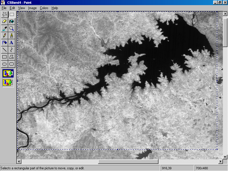
Figure 14: Paint window with cutout area.
Once the band has been converted to a bitmap format, it then can be opened into Paint. In Paint, pan to the section of the image which shows the entire reservoir. It is this portion of the image that will be cut out and analyzed. In the toolbox, click on the dashed line rectangular box and starting in the upper left corner, click and drag the mouse until the rectangular box has covered an area of 700 elements by 480 lines. Make sure that the entire reservoir is included in the box. It might be necessary to draw the box more than once to get the reservoir. The size of 700 elements by 480 lines can be determined by observing the coordinate values on the Status Bar when dragging the box across the image. See Figure 14. Do a copy of the subimage by selecting the “Copy” function under the “Edit” menu. This step will place the subimage in a temporary storage area called “Clipboard.”
Next under the “Image” menu, select the “Attributes” function. Change the width to 700 elements and the height to 480 lines. Now only the upper left portion of the full image is available. Click the “Edit” menu and then the “Paste” function. The subimage in “Clipboard” will now appear. Under the “File” menu, do a “Save As” and save the subimage in an appropriate directory. When saving the subimage, it is important to note if it is being saved as “256 Color Bitmap” file. See Figure 15. If it is not being saved in this format, an error has been made in the steps outlined above and it will be necessary to retrace them.
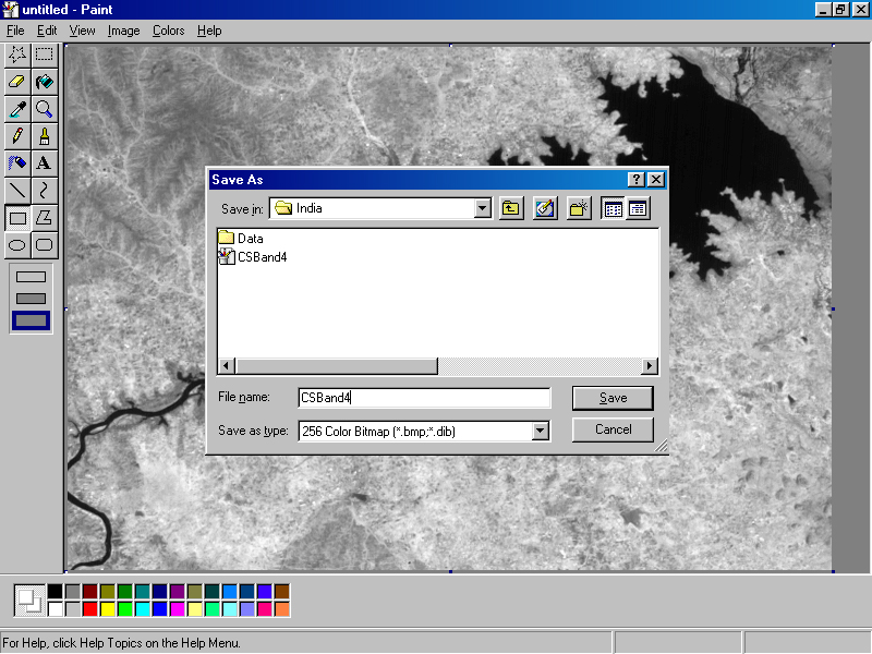
Figure 15: Subimage being saved in 256 Color Bitmap format.
After saving the subimage, it still appears on the Paint screen. The next step is to cut out the reservoir in more detail since some small water areas still exist throughout the subimage. In the toolbox a star shaped symbol appears. Click on this symbol. Holding down on the mouse, draw a line around the reservoir. It is not necessary to draw right along the edge of the water and it does not need to be real detailed. Once the reservoir has been encircled, release the mouse. Now do a “Copy” again under the “Edit” menu.
Now select the solid line box symbol on the toolbox. Three different boxes will appear. Click on the last one and select “white” on the color bar. Starting in the upper left corner, drag the mouse all the way to the lower right corner. The screen should now be completely white. Do a “Paste” under the “Edit” menu, and the cutout image should now appear. Finally, do a “Save As” and check again to make sure that the image is being saved in 256 Color Bitmap format. Figure 16 provides an example of the cutout image. The shape of the cutout area will vary. As long as it includes the reservoir and no other water areas, the shape of the cutout area is not crucial. The total file, which includes the white area, is still 700 elements wide and 480 lines high.
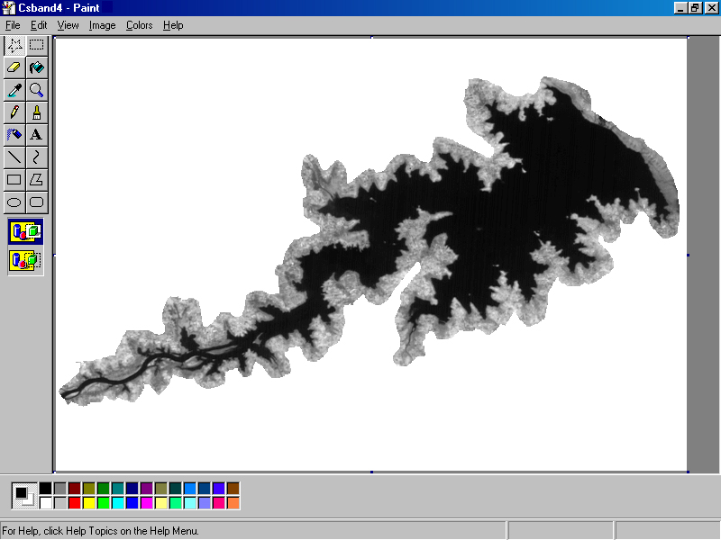
Figure 16: Cutout of the Tungabhadra Reservoir.
If one does not want to go through the procedure of developing a cutout of the reservoir, a cutout is included as a special data file with the data sets. The next major step is to move this file into EarthScenes and measure the surface area of the reservoir. Because this file is smaller than the original data set used in doing the synoptic analysis, a new file structure will have to be created under EarthScenes. Under the “File” menu, click “Import layer data for a new image” followed by “Create the data file for a new image.” Give a new name such as “TungaRes” to the new file structure and enter the size of the file which is 480 lines by 700 elements. Next under the “File” menu, click again “Import layer data for a new image” and then “Import BMP images.” Enter the cutout file and store it under layer 1. Do a “Create the histogram of a layer” under the “Enhance” menu. Under the “Display” menu, click the “Pixel read-out and zoom” function. Display the cutout image and move the mouse across the image taking note of the Z values. All of the white area should have values of 250. Move the mouse over the reservoir and take note of the Z values especially along the reservoir edge. Select what appears to be the highest Z value for water.
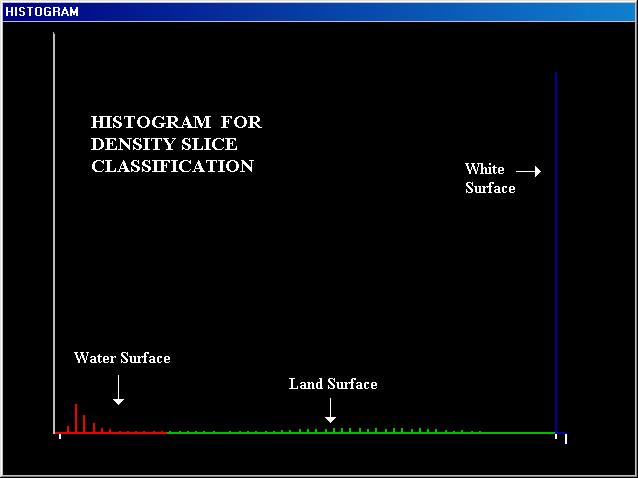
Figure 17: Annotated histogram of cutout image.
Once the highest Z value for water has been determined, the next step is to do a density slice classification of the cutout image. Under the “Classify” menu, select “Density Slice” followed by “Window and layer processing.” Select layer 1, the cutout image, as the input file and layer slot 2 as the output slot. It will be necessary to give an arbitrary name to the output layer such as “Density Slice Classification.” At this point a histogram will appear with instructions on how to slice the Z values into different classification ranges. There will be three classes: water, land, and white. Using the upper level Z value previously selected for water, press the “Ins” key on the keyboard. The color red should appear. Using the arrow key move across the histogram with the red color to the selected Z value. The author of this instructional module has picked “55” as the upper level Z value for water. Press the “Ins” key again at 55 and the color should change to green. Move the arrow key over to “249.” The Z values between “56” and “249” are displaying land conditions. Press the “Ins” key one more time and the color becomes blue. Move the arrow key across “250” to the end of the line and then press the “Del” key. Figure 17 illustrates the three classes on the histogram.
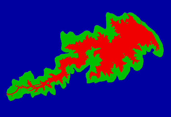
Figure 18: Density slice classification.
A layer similar to Figure 18 will be generated and stored in layer slot 2. Because it is stored, it can be viewed as many times as desired. Press the “Escape” button and a small window will appear with three numbers. These numbers represent the number of layer elements or pixels associated with the three classes. Based on the cutout image that the author developed and the Z values that he selected for the three classes, the numbers obtained were 47,526 for water, 52,652 for land, and 235,822 for white.
Knowing that each pixel covers 72.5 x 72.5m of Earth surface and that the reservoir is covered by 47,526 pixels, it is now possible to calculate the amount of water surface of the reservoir. A meter is approximately 3.28 feet. Multiply this number times 72.5 meters to determine the length in feet of the side of a pixel and then square that number to obtain the number of square feet in one pixel, which is 56,577.58. Next multiply this number by 47,526 to ascertain the total number of square feet of water surface. To obtain the number of acres, divide 43,560 (the number of square feet in an acre) into the total number of square feet of water surface. The number of acres should be about 61,728. Finally, divide this number by 640 (the number of acres in a square mile) to determine the number of square miles, which is 96.45. The reservoir at full capacity is 134.78 square miles. Thus, the water surface level in the reservoir is down by about 28 percent. Figure 19, a Landsat image taken on February 8, 1993, one day before the IRS image, shows that the water level in the reservoir has decreased significantly. All along the edge of the upper section of the reservoir a wide gray-colored rim exits, an area that would be covered by water during the monsoon season.
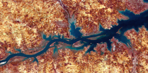
Figure 19: Low water level in upper portion of reservoir.
The satellite data used in this instructional module was taken
in the same year as the last hydrographic survey was conducted on the reservoir’s
storage capacity. Water surface area and storage capacity are two different
measurements of the water resources in the reservoir. However, water surface
data might assist in providing some indication of capacity during the intervening
years between when expensive hydrographic surveys are conducted.
REFERENCES:
Corbley, Kevin P. 1997. “Multispectral Imagery: Identifying More than Meets the Eye.” Geo Info Systems, June 1997.
Irrigation in Karnataka
http://waterresources.kar.nic.in/irri_in_kar.htm
Indian Weather
http://www.pbs.org/wnet/nature/monsoon/html/body_intro.html
Large dams and conflicts in the Krishna Basin
http://www.unu.edu/unupress/unupbooks/80a03e/80A03E0f.htm
Making of a Monsoon
http://www.pbs.org/wnet/nature/monsoon/html/body_make.html
Rain of Life and Death
http://www.pbs.org/wnet/nature/monsoon/html/body_rain.html
Reduction in the Storage due to Siltation and Attempts Made to Solve the Problem
http://www.tbboard.com/
River Systems of Karnataka
http://waterresources.kar.nic.in/river_systems.htm
The Indian Monsoon and Its Impact on Agriculture
http://www.usda.gov/oce/waob/jawf/profiles/specials/monsoon/monsoon.htm
Tungabhadra Project
http://www.tbboard.com/general.htm